
Keywords: Pivot Table, Chart, Data Form
Description: Learn how to use a pivot table as a source for a chart -- link a range of source data to the chart so that additions are automatically added to the chart.
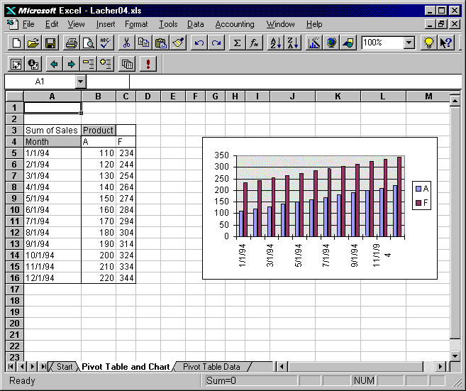
Tip: If you use a range of data as input to a pivot table -- and name that range " Database", the Data Form will add new records and include them in the named range. They will be included in the pivot table (after it is refreshed). You can link a chart to a pivot table so that changes in the pivot table automatically change the chart.
Guide to the Example: Worksheet "Pivot Table Data"
contains data range named "Database"....which is also
Pivot Table source range.
Chart on "Pivot Table and Chart" worksheet uses pivot
table as data source.
To demonstrate the advantages of this arrangement:
1. Use Data -> Form menu option to add new record to Pivot
Table Data. Excel automatically expands "Database"
range to include new data. Press refresh button on pivot table
worksheet and new data is automatically included in table.
2. Change pivot table by grouping data fields into quarters. Use
group button to automatically change monthly data into quarterly
data. Then hide the monthly data and chart will automatically
reflect new arrangement of data.
3. Move product pivot table field from its column position to be
a page field. Chart automatically adjusts and can be used to
chart each product.
Download File: Click Here
Tip: Click on the link above and choose
"Save" to download the xls workbook to your hard drive or "Open" to
open the workbook inside of your browser.
